IT Services

• ITS home
• Help
• Services
• My IT account
• About

Questions and answers

2227

How do I create a 'Supply and Demand' style chart in Excel?

If you need to produce a 'supply and demand' style chart using Excel, the following procedure for Excel 2010 could be useful:

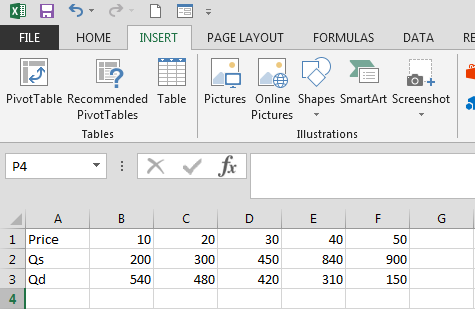
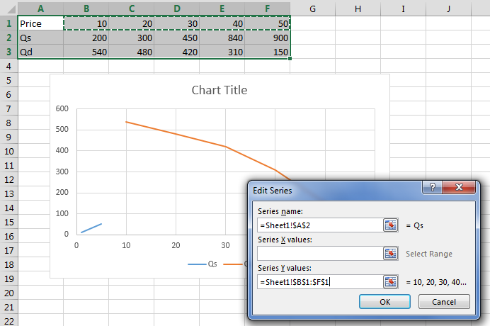
1. Open a new Excel spreadsheet and enter the data in a table as shown in this example.

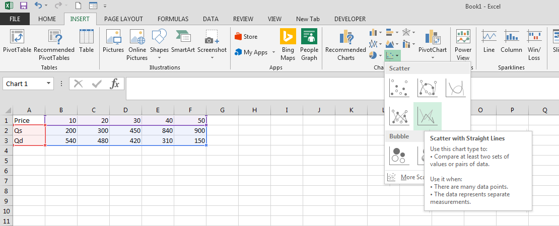
2. From the Insert tab, Chart group, choose Scatter and click on the icon for Scatter with Straight Lines (if you hover over the icon, the full description is shown).

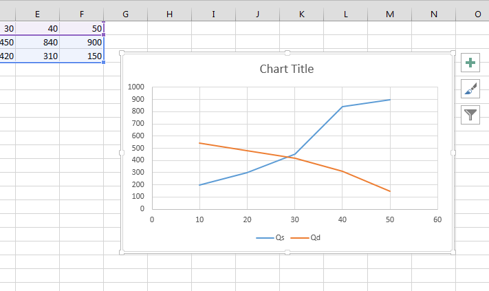
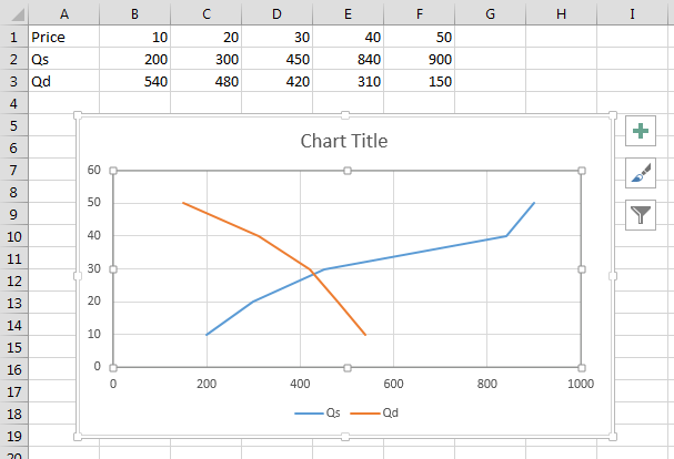
3. A chart will then appear with the familiar shape of the Supply and Demand diagram. However, the Price values are, by default, shown on the X-axis. The usual convention is to put the Price on the Y-axis and the following steps show how to switch the values around.

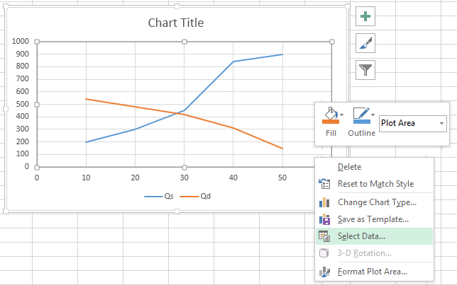
4. Right-click on the chart and choose Select Data from the mini menu.

5. Highlight the first row of data (Qs in this example) and then click on Edit.

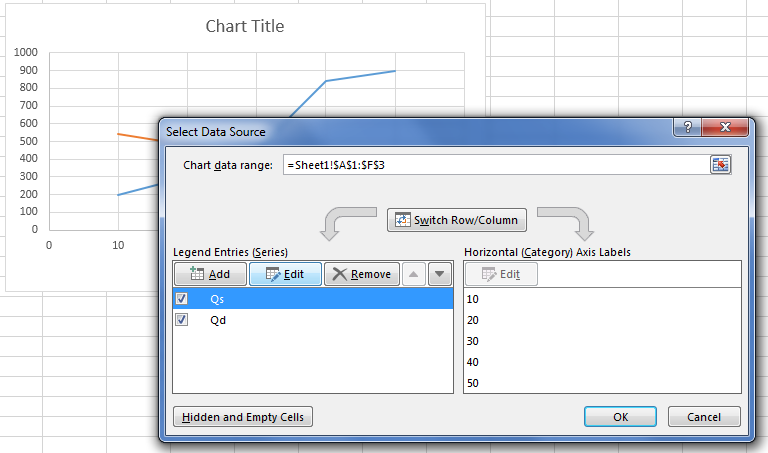
6. Delete the contents of the boxes for the X and Y axes.

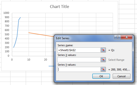
7. With the cursor in the box for the Y-axis values, highlight the price values in your table.

8. Now click into the box for the X-axis values and highlight the supply values in the table (Qs in the example shown) and click OK.

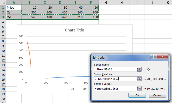
9. Repeat steps 5 to 8 for the second row of data (Qd) and when you click on OK, you will see that the chart has been rearranged with values for Price listed on the Y-axis.